Results for linear movement with cork

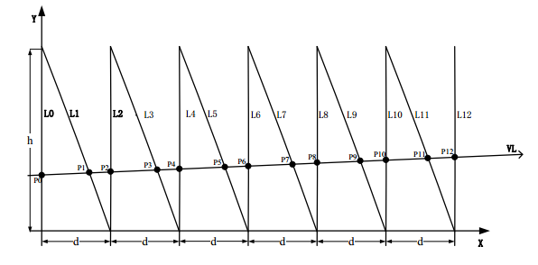
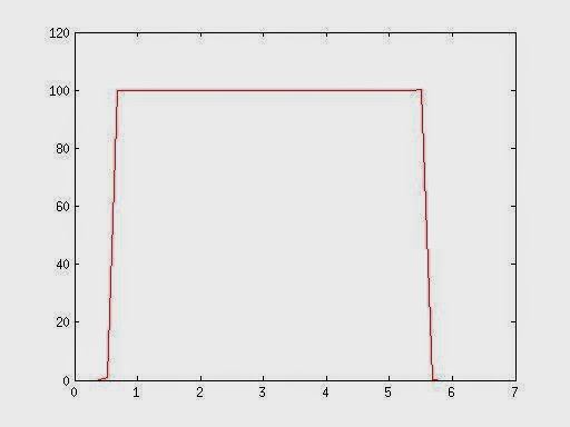
The first results are for a linear movement with a total of 500 mm with a constant speed of 100 mm/s. The velocity plot of the robot, the ground truth, is given below:

Figure 1 - Velocity (mm/s) vs Time (s)  of the robot (calculated at 5 Hz)

The total displacement measured by the robot was exactly 500 mm and after the acceleration phase the velocity is constant at 100 mm/s. Next, the results for the measurements with the camera will be shown, the results are for distances of 200, 300 and 400 mm.

Distance of 200 mm

At the distance of 200 mm the field of view was 50.5 mm. Below the results for the horizontal (0º) movement at 100 mm/s are shown:

Figure 2 - Measurements with the linear camera at 100 mm/s

At a frequency of 1250 Hz the results are very oscillatory, this is due to the slow movement and high sampling rate causing the consecutive frames to be very similar, causing problems on the correlation. At 500 Hz the result is the most similar to the ground truth, having a phase of constant velocity. At 250 Hz the correlation also showed some problems. The best results were at 500 Hz, next will be shown the plot of this camera measurement vs the robot.

Figure 3 - Robot vs Camera measurements 

As we can see, there is an error measuring the velocity, in the phase of constant velocity the error was 1,26%. The total displacement calculated by the camera was 493,4959 mm, giving an error of 1,3%.

Next are shown the results for the tests with oblique movement, in this case the error evolution is shown.

Figure 4 - Error evolution with the rotation of the camera sensor

There is a clear increase of the error with the increase of inclination in the movement, although this growth is small and the correlation works good.

Now the results for 500 mm/s:

Figure 5 - Measurements with the linear camera at 500 mm/s

At a frequency of 2500 Hz the result is the most similar to the ground truth, having a phase of constant velocity. At 1250 Hz the correlation also some problems having some reads with a higher value than the ground truth. At 500 Hz the results are very oscillatory, here the correlation method failed at some points due to the less overlap between frames. The best results were at 2500 Hz, next will be shown the plot of this camera measurement vs the robot.

Figure 6 - Robot vs Camera measurements

As we can see, there is an error measuring the velocity, in the phase of constant velocity the error was 1,26%, the same as at 100 mm/s. The total displacement calculated by the camera was 494,4329 mm, giving an error of 1,113%.

Next are shown the results for the tests with oblique movement, in this case the error evolution is shown.

Figure 7 - Error evolution with the rotation of the camera sensor

As seen at 100 mm/s, there is a clear increase of the error with the increase of inclination in the movement, although this growth is small and the correlation works good.

Distance of 300 mm

At the distance of 300 mm the field of view was 80.27 mm. With the horizontal (0º) movement at 100 mm/s are shown the velocity plots were very similar to the ones taken at 200 mm, although at 300 mm the best results was at 100 Hz. In the phase of constant velocity the error was 1,9%. The total displacement calculated by the camera was 509.0561 mm, giving an error of 1,811%.

At 500 mm/s the velocity plots were also very similar to the ones taken at 200 mm, the best results were at 500 Hz. In the phase of constant velocity the error was 1,9%, the same as before. The total displacement calculated by the camera was 508.2722 mm, giving an error of 1,6544%.

The error growth was also similar in both velocities.

Methodology

To prove that measuring velocity of a vehicle with a linear camera is possible, it is necessary to do measurements of movements and compare it with the ground truth. A industrial robot will be used for this purpose. The robot is well calibrated and has a very accurate positioning system, thus its movement is taken as ground truth. The robot gives its position data through a TCP/IP connection to a C++ client application. This application also calculates the time-stamps, later the velocity is calculated with this information. The acquisition rate is limited to 5 Hz due to the communication settings in the robot server.

In the first phase the movements will be simple linear movements and with constant velocity. Measurements will be done with the camera sensor horizontal to the movement and next measurements with the sensor oblique to the movement. Oblique movements can happen in the real world when the vehicle has perpendicular component on its movement, also it can happen when the camera isn't well installed. When the sensor has an angle with the direction of movement the frames will be captured as shown in the figure 1, the consecutive frames will have less similarity and is the correlation expected to be weaker, this will be one of the sources of error.

Figure 1 - Frames captured in an oblique movement

There will be made experiments at 100 mm/s and 500 mm/s, each of which will have measurements with the sensor at 0 degrees (horizontal), 2, 5 and 10 degrees of rotation to induce the oblique movement.

Experimental Procedure 

The experimental procedure for this first phase is described as follows:

• Camera positioning - The camera is positioned at the working distance from the robot;
• Focus adjustment - The optics focus is adjusted until the lines are clearly visible;
• Camera calibration - The angle of the camera is adjusted until the distance between the pairs of lines is equal, after this the camera will be horizontal to the movement and the field of view is determined. After this step the camera will not be moved anymore;
• The “ground” material in installed on the robot and the working distance is adjusted to compensate the thickness of the material. The distance is compensated adjusting the robot position;
• The measurements are made with the different velocities and angles of movement;
• This procedure is repeated to the other distances;

Ground Materials

The materials that will be used as ground will be cork, concrete, stone simulating pavement and cloth. With this material is possible to simulate a broad kind of textures. Fine grain textures with the concrete,  gross grain textures with the stone simulating pavement, textures with high variation with the cork and regular repetitive textures with the cloth.

Lighting

In the first tests was discovered that the light from the sun has a high influence on the image brightness and with this influence the captured image had a big brightness fluctuation throughout the day. To solve this problem and to have constant condition throughout the day the sun light was blocked in the lab. Instead artificial light will be used, the lighting will be done with two 500 W spotlights to provide enough brightness on the scene.

Velocity

Due to safety issues the robot will be used at a maximum of 500 mm/s. The robot base is not fixed on the ground and high velocities should be avoided.

Frame Rate

The maximum frame rate to be used in the experiments will be 2500 Hz. With this camera it cant be higher than that or the image will have lack of brightness due to low exposure times. For higher frame rates another camera should be considered.

First Test

This first test was made to assure that all the procedures are getting rightly done. This test was made with linear movement with total of 500 mm, horizontal to the camera sensor. The distance from the tip of optics to the "ground" was 200 mm and the velocity of the movement was 200 mm/s with a phase of acceleration at the beginning and deceleration at the end. The positions of the manipulator and the instants are registered through a Ethernet connection and simultaneously another computer does the frame's acquisition. The acquisition was set at 5000 Hz line rate. 

The texture used as "ground" was a piece of cork, as shown on figure 1, this texture is composed mostly of fine grain and should, in theory, represent a hard texture to find matches.

Figure 1 - Texture used as ground.

The calibration was done using the pattern described in the previous post. In the figure 2 there is presented one of the trials of the calibration process, the camera was adjusted until the spaces between the pairs of lines were all equal to assure that the sensor is truly horizontal to the movement of the robot. The field of view in this experiment was 51 mm.

Figure 2 - Process of the camera calibration

Two methods of correlation between consecutive frames were implemented. The Pearson product-moment correlation coefficient, used by [1] and the cross-correlation method using Fast Fourier transform, highly used in signal processing. Both the methods showed good results, although Pearson's correlation method has a high computational cost, so the cross-correlation method is the most suitable to process high quantity samples.

Results with the camera

With the sample of 5000 Hz were made various tests, one using the full sample at 5000 Hz, one at 2500 Hz, 1000 Hz, 500 Hz and 100 Hz.

At 5000 Hz the velocity calculated at all instants was zero, this is due to the very high sampling rate which caused the consecutive line to be very similar to the previous one and thus the pixel displacement to be zero. 

The results of the other tests made with the camera are shown below:

Velocity (mm/s) Vs Time (s) calculated at 2500 Hz

Velocity (mm/s) Vs Time (s) calculated at 1000 Hz

Velocity (mm/s) Vs Time (s) calculated at 500 Hz

Velocity (mm/s) Vs Time (s) calculated at 100 Hz

And the total displacement calculated is listed in the following table, the real displacement measured by the robotic manipulator was 500 mm.

Sample Rate [Hz]	Total Displacement [mm]
5000	0
2500	602.8706
1000	498.0863
500	498.0365
100	488.6283

[1] - "On modeling and control of omnidirectional wheels" by Viktor Kálmán

Camera Calibration

Camera calibration is a very important step, it is necessary to get the relationship between the object coordinates and the image coordinates. With known parameters of the camera model, including internal parameters and external parameters it is possible to determine this transformation. Calibration is used to determine this parameters. Camera matrix is one of the important internal parameters and position and orientation of the sensor to the world coordinate system are some of the important external parameters.[1]

In order to calculate the ground displacement from displacement between frames is necessary to know the relationship between the image size and the field of view size. Knowing this relation it is possible to calculate the real ground displacement at a given distance from the ground. The field of view is obviously dependent of the distance of the camera to the ground and for a better result it is essential to know this distance.

Therefore in a real implementation a method of estimating this distance should be available. In this work the test will be carried out with the help of a industrial robotic manipulator and his position will be used as ground-truth.

The experimental procedure proposed will require that the sensor is parallel to movement, the image being 1-D brings difficulties to assure that. To assure that the sensor is parallel to the movement a calibration method suggested by [1] [2] is used. The method implies the use of a pattern of vertical parallel lines crossed with diagonal lines, parallel with each other (figure 1)

Figure 1 - Pattern used for line scan cameras calibration [1]

With this configuration it is easy  to see that when the camera is completely horizontal the spaces between the pairs of lines will have an equal distance, and when the camera is oblique this spaces will have a tendency to increase or decrease depending on the orientation of the sensor. 

In the figure 2 is possible to see a image of the process of calibration, the image shown here is the representation of 480 repeated lines since the camera has not moved. The camera is adjusted until all the distances between the pairs of lines are equal. Once that is accomplished, the camera sensor is horizontal to the pattern and therefore horizontal to the movement.

Figure 2 - Image taken during the process of calibration.

[1] - "Line scan camera calibration for fabric imaging" by Zuyun Zhao

[2] - "Calibration of Line-Scan Cameras" by Carlos A. Luna, Manuel Mazo, José Luis Lázaro, Juan F. Vázquez

The Hardware

The hardware I will use on my work will be an industrial line scan camera. The model is P2-2x-04K40 from
Teledyne DALSA (figure 1).

Figure 1 - Line scan camera

The specifications of the camera are shown in the table 1. The output format is Camera Link, this imposes us some limitations, the acquisition will have to be on Windows workspace due to the lack of drivers. We only have access to the software provided by Teledyne DALSA and so we will have to capture the frames and posterior computational processing.

The camera has a very high speed and is highly configurable, it has the ability to work from 350 Hz to 36000 Hz and with a resolution from 128 to 4096 pixels.

Table 1 - General Camera Specifications

Resolution	4096 x 1
Max. Line Rate	36 kHz
Pixel Size	10 µm
Output Format	Camera Link Base